Disjoint Set

This is an example of a disjoint set:{1, 2, 4}, {5}, {7, 8}. There are 3 sets in total, wich each one containing various elements. Note that no element is present in more than one set, making the collection of sets ‘disjoint’ from one another.

A disjoint set supports the following operations:

Disjoint sets can be used to solve various problems quickly, an example given below:

Given an undirected graph $G$, perform $Q$ operations, either of Type A or B.

Type A: Create a bidirectional edge $(U,V)$ connecting vertices U, V

Type B: Determine whether vertices $U,V$ are connected to each other

Explanation

To keep track of the various elements in each set, a disjoint set appoints an arbitrary element from each set to act as the ‘representative’ of the entire set. Each set can now be represented as a rooted tree, with the representative of the set acting as the root.

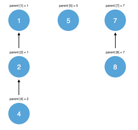
In the tree, each element is connected to another element, with the exception of the root, which is connected to itself. Only elements belonging to the same set will be connected to each other. To keep track of the various connections, a parent array is used, where parent[e] represents the parent element of e.

An example is shown below, representing the collection of sets {1, 2, 4}, {5}, {7, 8}:

Implementation

When initializing the disjoint set, it is assumed that all elements are initially in their own set. This can be implemented as follows:

// there are N elements in the disjoint set, numbered 0 to N - 1
int[] parent = new int [N];
// root[e] stores the relative depth/number of elements in the tree rooted at e
// this is used to implement the union() operation, and will be explained later
int[] rank = new int [N];

// each element is the root of its own tree and they all have the same rank at first (as each set contains one element)
for (int n = 0; n < N; n++) {
	rank[n] = 0;
	parent [n] = n;
}

Using this ‘rooted tree’ structure, it is simple to find which set a given element belongs to, i.e. the find() operation. Using DFS, we can traverse up the tree of the given element until the root is found, and returned.

// returns the root element of the set containing e
int find(int e) {
	// if root has not been found, keep recursing
	if (parent[e] != e) {
		// parent[e] links directly to root now, saving time for later operations
		parent[e] = find(parent[e]);
	}
	return parent[e];
}

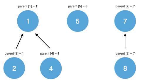
Note that the find() operation modifies the elements to link directly to the root of the tree for faster access in the future. For example, if find(4) is called on the above graph, the tree is modified as illustrated below:

Implementing the union() operation is also relatively easy. To merge the sets containing e1 and e2, the roots of the trees containing e1 and e2 must be found. If the roots are identical, e1 and e2 are already in the same set and no work needs to be done.

Otherwise, the root of the larger tree will become the root of the smaller tree. This is done to improve the performance of the find() operation on elements of the smaller tree (as less parent values will have to be updated to account for the new root of the tree).

But how do we know which tree has more elements? In order to always assign the smaller tree to the root of the larger tree, a second array, rank, will be used, where rank[e] represents the ‘depth’ of the tree rooted at e (relative to the other trees).

If rank[e1] > rank[e2], this means that e1 is part of a larger tree than e2, and that parent[find(e2)] should be assigned to find(e1).

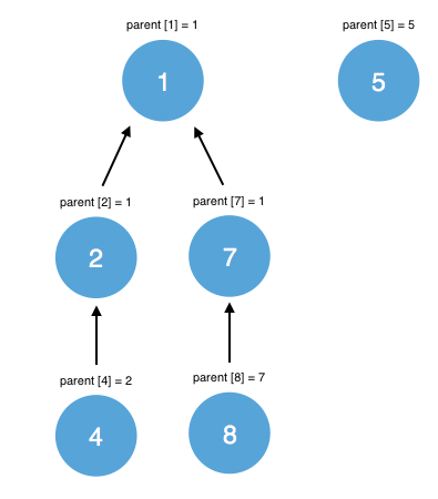
The result of the operation union(4, 7) on the original example is shown below:

The ideas discussed above are implemented below:

// merges the sets that contain e1 and e2
void union(int e1, int e2) {
	int root1 = find(e1), root2 = find(e2);

	// e1 and e2 are already part of the same set, nothing should be done
	if (root1 == root2)
		return;
	
	if (rank[root1] < rank[root2]) {
		// if tree rooted at root1 is longer than root2
		parent[root1] = root2;
	} else if (rank[root1] > rank[root2]) {
		// if tree rooted at root2 is longer than root1
		parent[root2] = root1;
	} else {
		// the roots have the same rank, doesn't matter which one becomes the new root
		// as the new tree has a greater max depth now, increase the rank of the new root by 1
		parent[root1] = root2;
		rank[root2]++;
	}
}

Time Complexity

Construction: $O(N)$, where $N$ is the total number of elements.

Find operation: nearly $O(1)$ amortized, explanation of this is beyond the scope of this lesson.

Union operation: nearly $O(1)$ amortized, explanation of this is beyond the scope of this lesson.

Space Complexity

$O(N)$, where $N$ is the total number of elements.

Conclusion

The disjoint set is a powerful data structure which can perform find() and union() operations in near constant time. Using disjoint sets, the solution to the given problem can be implemented in approximately $O(N+Q)$ time.

Practice

Disjoint Set Test