This content is archived!
For the 2018-2019 school year, we have switched to using the WLMOJ judge for all MCPT related content. This is an archive of our old website and will not be updated.Notation
Big O notation looks like a math function: \mathcal{O}(1)
The contents of the brackets represents the performace. Variables may be used. Generally, the variable N is used, however, more variables may be needed and some may be defined in a problem given. It is convention to use a single letter as a variable. We prefer uppercase ones.
Big O describes the worst-case scenario or at least a plausible worst-case. This makes it easier to quantify the complexity.
Another rule is that only the dominating factors are used. This means that coefficients and lower order terms are discarded.
Determining Complexity
Complexity is determined by analyzing the number of operations an algorithm performs or the amount of memory allocated by a data structure. For example, if a program looks like the following, then the complexity is \mathcal{O}(N)
for (int n = 0; n < N; n++) {
	// Do something in O(1)
}
Similarly, the following is \mathcal{O}(NM)
for (int n = 0; n < N; n++) {
	for(int m = 0; m < M; m++) {
		// Do something in O(1)
	}
}
\mathcal{O}(1) is something such as doing an addition operation, accessing a variable, etc.
Logarithmic complexity (\mathcal{O}(\log N)) typically comes from some kind of binary search.
Common Complexities
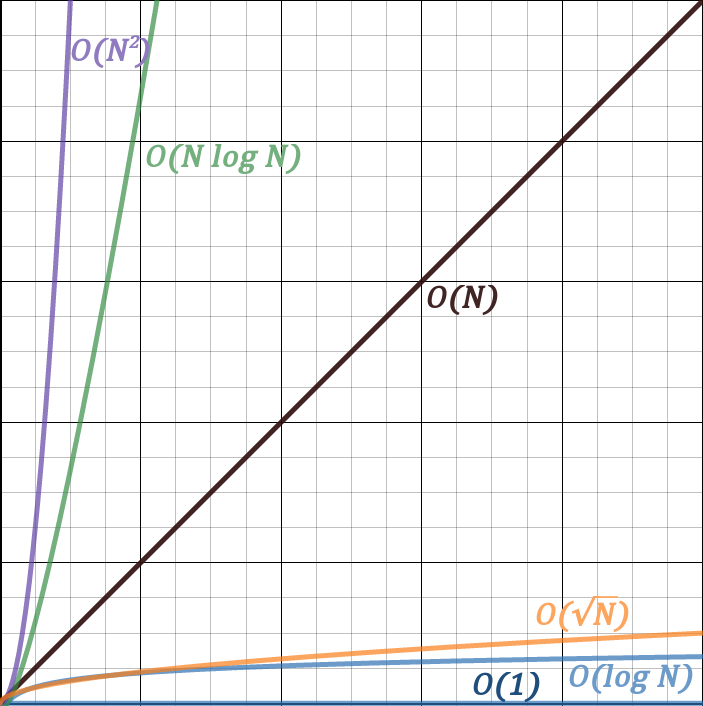
We will now compare many common complexities. The upper bound on both axes is 100.
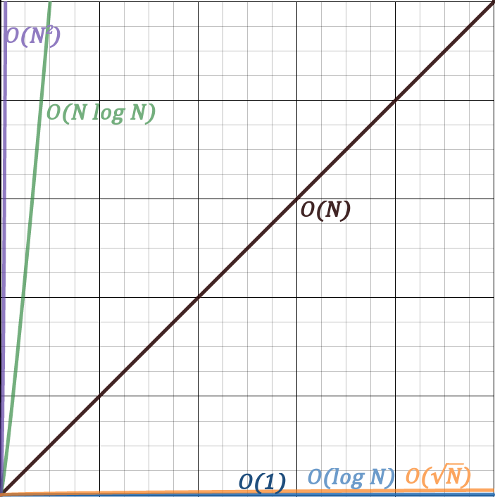
Now this is the same graph except on a bigger scale. The upper bound on both axes is 10000.
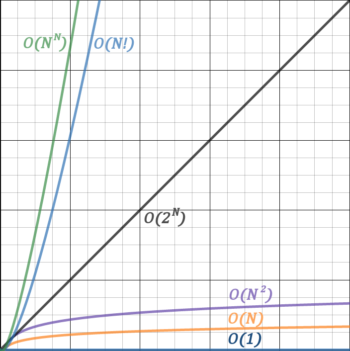
However, there are a couple of complexities that aren’t didn’t include here because they grow too quickly to be graphed. We will look at them on a logarithmic scale. The upper bound on both axes is 100.
Constraints
Knowing the maximum constraint of an algorithm is a useful in figuring out the time complexity required to solve a given problem.
In the following is a table, the first row contains the maximum values N that a given complexity can handle with the assumption that the computer can handle {10\,000\,000} operations per second and that you only have a second of run time. The second row contains the number of operations given N=100. Actual benchmarks may differ depending on the system. The table is an approximation.
| Complexity | Maximum Value | Operations (N=100) | Examples |
|---|---|---|---|
| \mathcal{O}(1) | N/A | 1 | Accessing memory, doing simple math, etc. |
| \mathcal{O}(\log N) | 10^{3\,000\,000} | 7 | Performing a binary search, using a map or set (both binary search trees). |
| \mathcal{O}(\sqrt{N}) | 10^{14} | 10 | Checking a prime number or prime factorization. |
| \mathcal{O}(N) | 10^{7} | 100 | An iterative search, a for loop, an iteration, etc. |
| \mathcal{O}(N\log N) | 1\,600\,000 | 665 | Sorting. Using a map or set on N elements. |
| \mathcal{O}(N^2) | 3\,000 | 10\,000 | Most naive sorting algorithms, and absolute worst-case of good ones. |
| \mathcal{O}(N^2\log N) | 1\,700 | 66\,439 | Rarely encountered, no useful examples. |
| \mathcal{O}(N^3) | 200 | 1\,000\,000 | Three nested for loops. 3D DP. |
| \mathcal{O}(N^4) | 56 | 100\,000\,000 | Four nested for loops. 4D DP. |
| \mathcal{O}(2^N) | 23 | 10^{30} | Finding subsets, bitmasking, combinations. |
| \mathcal{O}(N!) | 10 | 10^{158} | Combinatorics (permutations) and brute force. |
| \mathcal{O}(N^N) | 8 | 10^{200} | Combinatorics (permutations). |